Chunk 51 Submitted

A Curve Example 1

The previous chapter (Chapter X) showed us how to draw a curve made by a ball falling under the effects of gravity. A constant speed was applied to the x-axis and a constant acceleration, gravity, was applied to the y-axis. But what if we want to draw curves that have bends in them? To do that, we need to replace the constant acceleration with variable acceleration.

In this chapter we will explore two example curve drawing programs. The first, 'Hills', will produce a bendy curve by varying y-axis acceleration, and the second example, 'Fly in a Room', will draw a more elaborate curve by applying varying acceleration to both the x- and y- axes.

Acceleration & Deceleration

In nature, acceleration and deceleration are forces that cause objects to change their speed. Acceleration causes objects to move faster and faster as time goes by, whereas deceleration causes objects to move progressively slower. Acceleration is made up of two components: (1) its size and (2) its direction. When a car driver presses her foot down on the accelerator pedal the car is subjected to an acceleration whose size is proportional to how far down the pedal is pressed and whose direction is forward as viewed by the driver. And, if the same driver engages the car's reverse gear and presses the accelerator then the car is accelerated backwards.

Mathematically, if we use positive numbers to represent accelerations in the forward direction then negative numbers represent accelerations in the backward direction. For example if an acceleration of 10 represents that a car accelerates forward by ten miles per hour for each second that passes, then a value of -2 will denote that the car accelerates backwards, or decelerates, by two miles per hour per second.

Considering that both an acceleration's size and direction are important and that Processing's coordinate system results in higher y-axis values representing positions lower down the drawing window (see Chapter X), we need to agree on terminology that will help us avoid confusion. In this chapter, we will stick to using the terms upward acceleration and downward acceleration as described in the below table.

              What Does         What Does it         
              it Mean           it Mean          Acceleration
Term          Visually?         Mathematically?  Value
-------------------------------------------------------------
Downward      Causes y-values   Causes y-values  Positive
Acceleration  to denote         to INCREASE 
              positions closer  in value.
              to the drawing 
              window's
              BOTTOM edge.
-------------------------------------------------------------
Upward        Causes y-values   Causes y-values  Negative
Acceleration  to denote         to DECREASE
              positions closer  in value.
              to the drawing 
              window's
              TOP edge.
-------------------------------------------------------------

The example programs presented in this chapter need to generate upward and downward accelerations that have randomly chosen sizes. To do this the examples use the code similar to that which is shown below. In this case, the random() function returns a random number between 0.2 and 0.8 inclusive and the minus sign (-) is used to convert the positive number returned by random() to a negative number.

float downwardAcceleration=random(0.2,0.8);
float upwardAcceleration=-random(0.2,0.8);

Hills

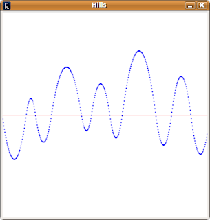
The 'Hills' example program draws a bendy curve that mimics the outline made by a range of hills (see Figure 1). The program starts halfway down the left-hand side of the drawing window and draws a curve across to the right hand-side. The program applies a constant speed to the x-axis and a varying acceleration to the y-axis. The y-axis acceleration is changed each time the y value passes the y-axis centre-line – an imaginary horizontal line halfway down the drawing window. Each time the y value passes the centre-line the program changes the direction of the acceleration so that it is always towards the centre-line – when the y value is above the centre-line the acceleration is set to be downward and vice-versa.

Figure 1: The 'Hills' program. The curve drawn in blue is drawn by the program. The y-axis centre-line has is shown in red as a guide.

The complete 'Hills' program is shown below.

// Setup the drawing window
size(400,400);
background(255);
smooth();
strokeWeight(2);
stroke(0,0,255);

// Set initial values for variables
int yCentre=height/2;
int y=yCentre;
float ySpeed=8;
float yAcceleration=-random(0.2,0.8);

// Main loop: Increment x from left-hand side of window to right-hand side.
for(int x=0;x<width;x++)
{
 // When y passes up through the y-axis centre-line,
 // randomly choose a new downward acceleration.
 if(y<yCentre && yAcceleration<0) yAcceleration=random(0.2,0.8);

 // When y passes down through the y-axis centre-line,
 // randomly choose a new upward acceleration.
 if(y>yCentre && yAcceleration>0) yAcceleration=-random(0.2,0.8);
  
 // Update y value and draw point
 ySpeed+=yAcceleration;
 y+=ySpeed;
 point(x,y);
}

The first section of the program sets up the drawing window so that it's 400 by 400 pixels, has a white background and drawing is done in blue.
The second section (see below) sets the initial values of the variables that are used to draw the curve. The value of y is set to be halfway down the drawing window, the value of ySpeed is set to be 8 and yAcceleration is set to be an upward acceleration with a size of between 0.2 and 0.8.

int yCentre=height/2;
int y=yCentre;
float ySpeed=8;
float yAcceleration=-random(0.2,0.8);

The third and final section of the program contains the main loop which draws a point for each of the pixels that make up the width of the drawing window. The loop is a for..next loop (see Chapter X) that increments x from the left-hand side of the drawing window to the right-hand side in increments of one pixel. In other words, x is incremented from 0 to 399 and the body of the loop is iterated a total of 400 times.

for(int x=0;x<width;x++)
{
...
}

Inside the main loop are the parts of the program that:
(1) vary the acceleration when the y value passes the centre-line,

if(y<yCentre && yAcceleration<0) yAcceleration=random(0.2,0.8);
if(y>yCentre && yAcceleration>0) yAcceleration=-random(0.2,0.8);

(2) that updates the values of ySpeed and y,

ySpeed+=yAcceleration;
y+=ySpeed;

and (3) draws the point at the coordinates x, y.

point(x,y);

Fly in a Room

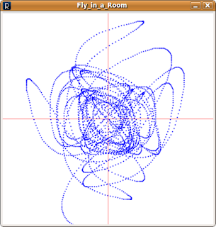
The 'Fly in a Room' example program is an extension of the 'Hills' program. Instead of applying a varying acceleration to the y-axis, the 'Fly in a Room' example applies varying accelerations to both the x- and y- axes. The result is a bendy curve that looks somewhat like the path of a fly trying to escape a room (see Figure 2).

Like the 'Hills' program, this example considers each axis has a centre-line and varies accelerations so that they point towards the centre-lines. The x-axis acceleration will always be in the direction of the x-axis centre-line and likewise with the y-axis acceleration pointing to the y-axis centre-line. The sum of the x- and y-axis accelerations result in an acceleration that always points to the centre of the display window. Unlike the 'Hills' program, this example starts drawing not on the left-hand side of the drawing window but in its centre.

So how does the fly escape the room? Well, even though the accelerations are always pointing towards the centre of the display window sometimes strong accelerations will cause the x, y position to shoot past the centre point and end up outside of the display window. When that happens the program is configured to stop drawing and to show the display window to the viewer.

Figure 2: The 'Fly in a Room' program. The curve drawn by the program is shown in blue. The x- and y-axis centre-lines are shown in red as a guide.

The complete 'Fly in a Room' program is given below.

// Setup the drawing window
size(400,400);
background(255);
smooth();
strokeWeight(2);
stroke(0,0,255);

// Set initial values for variables
int yCentre=height/2,xCentre=width/2;
int y=yCentre,x=xCentre;
float ySpeed=4,xSpeed=4;
float yAcceleration=-random(0.1,0.4),xAcceleration=-random(0.1,0.4);

// Main loop: Continue drawing until either the x or y value becomes outside the
// drawing window.
while(y>0 && y<height && x>0 && x<width)
{
 // Vary y-axis acceleration when y-axis centre-line passed.
 if(y<yCentre && yAcceleration<0) yAcceleration=random(0.1,0.4);
 else if(y>yCentre && yAcceleration>0) yAcceleration=-random(0.1,0.4);

 // Vary x-axis acceleration when x-axis centre-line passed.
 if(x<xCentre && xAcceleration<0) xAcceleration=random(0.1,0.4);
 else if(x>xCentre && xAcceleration>0) xAcceleration=-random(0.1,0.4);

 // Update x and y values and draw point
 ySpeed+=yAcceleration;
 y+=ySpeed;
 xSpeed+=xAcceleration;
 x+=xSpeed;
 point(x,y);
}

In theory, because the x and y values depend on random numbers it is possible that the main while loop (see Chapter X) will continue forever. Although, in practice when the program is run it has always terminated and displayed the drawing window to the user. If we wanted to ensure that the program does always terminate within a reasonable amount of time, we can introduce a time clause to the program's central loop. The below code shows how the while loop can be changed to ensure that the loop does not continue for more than one second (1000 milliseconds).

int startTime=millis();
while(y>0 && y<height && x>0 && x<width && millis()-startTime<1000)
{
...
}

First Thoughts

Wow. I was expecting Processing to be a graphics library that could be used by Java programs. Instead it's an IDE with an in-built interpreter for the Processing language. 

I am guessing that in reality the core of Processing has been implemented as set of Java classes and that the 'interpreter' is actually a pre-processor that translates the Processing code into Java code.

If my guess is correct, the approach reminds me of JSP pages which are pre-processed into implementations of the HttpServlet Java class before being compiled and executed.